library(tidyverse)
library(fpp3)

# Code block 1: FPP 9.4 Fig 9.6 a) -----
# Errors
epsilon <- rnorm(n=100, mean=0, sd=1)

# Store values of yt here
yt <- rep(0, times = 100)
yt[1] <- 20
for(t in 2:100){
  yt[t] <- 20 + epsilon[t] + 0.8*epsilon[t-1]
}
plot(yt, type = 'l')


# Code block 2: FPP 9.5 example (in different order) ------
# Load data
egypt_exports <- global_economy |>
  filter(Code == "EGY") %>%
  select(Year, Exports)
egypt_exports

# Visualize raw data:
egypt_exports |>
  autoplot(Exports) +
  labs(y = "% of GDP", title = "Egyptian exports")

# Visualize autocorrelation function:
egypt_exports %>%
  ACF(Exports) %>%
  autoplot()

# Visualize partial autocorrelation function:
egypt_exports %>%
  PACF(Exports) %>%
  autoplot()

# Fit ARIMA(p,d,q) where you instead of specifying (p,d,q), you let function
# find these values for you
fit <- egypt_exports |>
  model(ARIMA(Exports))

# Get model fitted parameters
report(fit)

fit |>
  forecast(h=10) |>
  autoplot(egypt_exports) +
labs(y = "% of GDP", title = "Egyptian exports")SDS390: Ecological Forecasting
Lec 15.2: Thu 12/14
Announcements
- Fill out course evals
- Deadlines:
- Today
5pm9pm: 5min video presentation on Moodle - Mon 12/18 8am: Feedback on video presentations returned by Prof. Kim
- Thu 12/21 3pm: Final version of notebook due on Moodle
- Today
Today
- Model validation:
- Train/test splitting: Only when you want an estimate of prediction/forecasting error of \(y\) vs \(\widehat{y}\) into the future. Most typical measure of error is Root Mean Squared Error (RMSE); we took the square root so that units of error measure match units of \(y\)
- Residual analysis. Typically done on all data (no train/test split), used to verify:
- Assumptions required to ensure p-values and confidence intervals are valid
- No pattern in residuals. In the case of time series analysis, you also need to run ACF of residuals to ensure there is not autocorrelation
- Sum of squared error \(\sum_{i=1}^{n}\left(y_i - \widehat{y}_i\right)^2\): Measure of model quality based only on lack of fit of \(\widehat{y}\) to \(y\). This is quantity minimized by many regression methods
- AIC/BIC: Measure of model quality that balances lack of fit of \(\widehat{y}\) to \(y\) and model complexity. Guards against overfitting (on slide 20).
- Work on final project
Closing thoughts
- 24J grads?
- Time series: Made it to ARIMA, even if there were gaps
- Python
- Remember my thoughts about ChatGPT. It is a very powerful tool, but you need to be:
- Knowledgeable enough to understand the code
- Experienced enough in your domain and programming to know what to prompt
- Disciplined enough to sanity check your results
- Small class upper level classes: can take risks
- Thank you for your flexibility; recall what I wrote in the syllabus: to the extent you can show me patience and grace, I will return the favor.
Lec 15.1: Tue 12/12
Announcements
- I posted PS1-PS3 and DC grades. If you’ve completed all 4 DC courses but didn’t get 4/4, please let me know; you might have one or two exercises that aren’t 100% completed.
- Deadlines:
- Thu 12/14 5pm: 5min video presentation on Moodle
- Mon 12/18 8am: Feedback on video presentations returned by Prof. Kim
- Thu 12/21 3pm: Final version of notebook due on Moodle
Lecture
- Work on final project
Lec 14.2: Thu 12/7
Announcements
Lecture
- PS4 in-class
- FPP 9.9 Seasonal ARIMA. Use 4th DC Chapter 4 as reference
Lec 14.1: Tue 12/5
Announcements
- While there is no explicit lecture today, class is not cancelled. Please:
- Meet with your partner to work on final project
- Take a group selfie proving you met up to work. This will count to your participation/engagement grade
- Create a Slack DM that has all group members + me and send me the photo
- If you’re the only one of your group members to make it to class, please take a selfie of just yourself.
- PS4 presentations on Thursday. Please re-read instructions on Problem Sets page.
- We’re done DC courses, but if you have the energy at some point it might be worth completing the 5th course in the Time Series with Python track on Machine Learning for Time Series Data. If you do, you’ll get a Statement of Accomplishment, which may help you during job searches
Lec 13.2: Thu 11/30
Announcements
- Office hours start late today: 11:30am - 12:05pm
- Class on Tuesday
Lecture
- FPP 9.3 Autoregressive model: Specific cases of AR(1) model
- FPP 9.4 Moving Average modeling (recall: this is not moving average smoothing)
- FPP 9.5 Non-seasonal ARIMA models
- FPP 9.7 Modeling procedure
Lec 13.1: Tue 11/28
Announcements
- PS4 attendance policy
- Final project added instructions
Lecture
- FPP 9.1 Stationarity and differencing
- FPP 9.2 Backshift notation
- FPP 9.3 Autoregressive model
library(tidyverse)
library(fpp3)
library(patchwork)

# Code block 1: Fig 9.1 a) and b) data Google Stocks
google_2015 <- gafa_stock |>
  filter(Symbol == "GOOG", year(Date) == 2015)

# Not stationary:
google_2015 %>% autoplot(Close)

# Differences are stationary:
google_2015 %>% autoplot(difference(Close))

# Compare autocorrelation functions:
plot1 <- google_2015 %>% ACF(Close) %>% autoplot()
plot2 <- google_2015 %>% ACF(difference(Close)) %>% autoplot()
plot1 + plot2


# Code block 2: FPP 9.3 Fig 9.5a) Simulate 100 values of AR1 process
AR1_ex <- rep(0, 100)

# Set first value
AR1_ex[1] <- 11.5

for(t in 2:100){
  # Intercept 18 + slope of previous obs -0.8 + epsilon random noise
  AR1_ex[t] = 18 - 0.8*AR1_ex[t-1] + rnorm(n=1, mean=0, sd=1)
}
plot(AR1_ex, type = 'l')
Lec 12.1: Tue 11/21
Announcements
- No in-class lecture
- Final project extra notes
- Fit between 2-4 models, one of which needs to be an ARIMA model
- Do a residual analysis of the model selected for forecasting into the future using all the available data
Lecture
- Recorded lecture posted in Screencasts tab of webpage (top right). Please post questions in Slack under
#questionsincluding the point in time in video your question corresponds to. Topics:- FPP 8.2 Exponential smoothing with trend
- FPP 8.3 Exponential smoothing with seasonality
- PS4 files posted on Slack, please read instructions on Problem Sets page
library(tidyverse)
library(fpp3)

# Code block 1: Example from FPP 8.2 on exponential smoothing with trend ----
# a) Get and visualize data
aus_economy <- global_economy |>
  filter(Code == "AUS") |>
  mutate(Pop = Population / 1e6)
autoplot(aus_economy, Pop) +
  labs(y = "Millions", title = "Australian population")


# b) Regular exponential smoothing with trend
fit <- aus_economy |>
  model(
    # Additive (i.e. non-multiplicative) error and trend, no seasonality:
    AAN = ETS(Pop ~ error("A") + trend("A") + season("N"))
  )

# Forecast ten times points into future
fc <- fit |>
  forecast(h = 10)

# NOT IN BOOK: get the fitted alpha/beta and l0/b0 values
# NOTE: CRAZY high alpha! Very high weight on previous observation!
report(fit)
tidy(fit)

# Fitted values in orange, forecasts in blue.
# Note:
# 1. Confidence band is narrow
# 1. Problem forecast increases forever into the future
fc |>
  autoplot(aus_economy) +
  geom_line(aes(y = .fitted), col="#D55E00", data = augment(fit)) +
  labs(y = "Millions", title = "Australian population") +
  guides(colour = "none")


# c) Dampened exponential smoothing with trend
fit <- aus_economy |>
  model(
    # Previous model: Additive (i.e. non-multiplicative) error and trend, no seasonality:
    # AAN = ETS(Pop ~ error("A") + trend("A") + season("N"))
    # Dampened model with given phi: Additive error, dampened trend with given phi parameter, no seasonality:
    # AAN = ETS(Pop ~ error("A") + trend("Ad", phi = 0.8) + season("N"))
    # Dampened model letting phi be estimated:
    AAN = ETS(Pop ~ error("A") + trend("Ad") + season("N"))
  )

# Forecast ten times points into future
fc <- fit |>
  forecast(h = 10)

# NOT IN BOOK: get the fitted alpha/beta and l0/b0 values
# NOTE: Another high value of alpha
report(fit)
tidy(fit)

# Fitted values in orange, forecasts in blue.
# Note:
# 1. How dampening parameter flattens out forecast curve.
fc |>
  autoplot(aus_economy) +
  geom_line(aes(y = .fitted), col="#D55E00", data = augment(fit)) +
  labs(y = "Millions", title = "Australian population") +
  guides(colour = "none")


# Code block 2: Example from FPP 8.3 on exponential smoothing with seasonality ----
aus_holidays <- tourism |>
  filter(Purpose == "Holiday") |>
  summarise(Trips = sum(Trips)/1e3)

autoplot(aus_holidays, Trips) +
  labs(y = "Thousands", title = "Australian trips")

fit <- aus_holidays |>
  model(
    # Additive and multiplicative models:
    #additive = ETS(Trips ~ error("A") + trend("A") + season("A")),
    #multiplicative = ETS(Trips ~ error("M") + trend("A") + season("M"))
    # Additive and multiplicative models with dampening:
    additive = ETS(Trips ~ error("A") + trend("Ad", phi = 0.2) + season("A")),
    multiplicative = ETS(Trips ~ error("M") + trend("Ad", phi = 0.2) + season("M"))
  )

# NOT IN BOOK: get the fitted alpha/beta and l0/b0 values
report(fit)
tidy(fit)

fc <- fit |>
  forecast(h = "3 years")

# Plot both models:
# NOTE
fc |>
  autoplot(aus_holidays, level = NULL) +
  labs(title="Australian domestic tourism",
       y="Overnight trips (millions)") +
  guides(colour = guide_legend(title = "Forecast"))
Lec 11.2: Thu 11/16
Announcements
- Residual analysis: on which data? train or test or both?
Lecture
- Simple exponential smoothing
library(tidyverse)
library(fpp3)

# Code block 1: Study weights in an exponential model ----
# Choose 0 < alpha <= 1
alpha <- 0.9
k <- 1:11

# Inspect and visualize weights:
alpha*(1-alpha)^(k-1)
plot(k, alpha*(1-alpha)^(k-1))

# As consider more and more weights, weights sum to 1
sum(alpha*(1-alpha)^(k-1))


# Code block 2: Example from FPP 8.1 ----
# Get and visualize data
algeria_economy <- global_economy |>
  filter(Country == "Algeria")
algeria_economy |>
  autoplot(Exports) +
  labs(y = "% of GDP", title = "Exports: Algeria")

# Fit simple exponential smoothing model using ETS() function:
# Additive, not multiplicative model. No trend or season for now.
fit <- algeria_economy |>
  model(ETS(Exports ~ error("A") + trend("N") + season("N")))

# NOT IN BOOK: get the fitted alpha and l0 values
report(fit)
tidy(fit)

# Forecast 5 time points into the future
fc <- fit |>
  forecast(h = 5)

# Fitted values in orange, forecasts in blue.
# Note:
# 1. LARGE forecast error interval
# 2. This is only simple exponential smoothing
# 3. Comparing orange and black lines, we see degree of smoothing is not that high
fc |>
  autoplot(algeria_economy) +
  geom_line(aes(y = .fitted), col="#D55E00", data = augment(fit)) +
  labs(y="% of GDP", title="Exports: Algeria") +
  guides(colour = "none")
Lec 11.1: Tue 11/14
Announcements
- PS3 mini-presentations today. Info in Problem Sets
- Finalized final project information posted in Final Project
Lec 10.2: Thu 11/9
Announcements
- In-class guest lecture today with Prof. Will Hopper
- Work on PS3. Note link to rendered output of all previous PS
.ipynbfiles have been posted in Problem Sets
Lec 10.1: Tue 11/7
Announcements
- Zoom lecture today starting at
regular class time10am (Zoom link sent on Slack) - Answer Poll Everywhere question in Slack
#generalon whether you prefer group or individual final projects - Discuss final project. Info in Problem Sets
Lec 9.1: Tue 10/31
Announcements
- No lecture on Thursday from Cromwell Day
- Zoom lecture on Tuesday 10/7
- In-class lecture on Thursday 10/9 with Prof. Will Hopper
Lecture
- Start PS3
Lec 8.2: Thu 10/26
Announcements
- Fill out PS2 peer eval Google Form and slido poll
Lecture
- FPP 5.5: Prediction intervals
- FPP 5.7: Forecasting with STL decomposition method
- FPP 5.8: Assessing prediction accuracy
Lec 8.1: Tue 10/24
Announcements
- PS2 mini-presentations today. Info in Problem Sets
Lecture
Lec 7.2: Thu 10/19
Announcements
- Update PS2 in-class presentation format in Problem Sets
- PS2 mini-presentations this coming Tuesday
Lecture
- Code blocks below
- Refresher on conditions for inference for linear regression
library(fpp3)

# Code block 1: Fit model to data and generate forecasts ----
# Tidy:
full_data <- aus_production %>%
  filter_index("1992 Q1" ~ "2010 Q2")

# Visualize:
full_data %>%
  autoplot(Beer)

# Specify: Take full data and fit 3 models
beer_fit_1 <- full_data |>
  model(
    Mean = MEAN(Beer),
    `Naïve` = NAIVE(Beer),
    `Seasonal naïve` = SNAIVE(Beer)
  )

# Generate forecasts 14 time periods (quarters) into future
beer_forecast_1 <- beer_fit_1 |>
  forecast(h = 14)

# Plot full data and forecasts
plot1 <- beer_forecast_1 |>
  autoplot(full_data, level = NULL) +
  labs(
    y = "Megalitres",
    title = "Forecasts for quarterly beer production"
  ) +
  guides(colour = guide_legend(title = "Forecast"))

plot1


# Code block 2: Training test set approach ----
# Define training data to be up to 2007: fit the model to this data
training_data <- full_data |>
  filter_index("1992 Q1" ~ "2006 Q4")

# Define test data to be 2007 and beyond:
test_data <- full_data |>
  filter_index("2007 Q1" ~ "2010 Q2")

# Fit 3 models only to training data
beer_fit_2 <- training_data |>
  model(
    Mean = MEAN(Beer),
    `Naïve` = NAIVE(Beer),
    `Seasonal naïve` = SNAIVE(Beer)
  )

# Generate forecasts for 14 quarters
beer_forecast_2 <- beer_fit_2 |>
  forecast(h = 14)

# Plot training data and forecasts only
plot2 <- beer_forecast_2 |>
  autoplot(training_data, level = NULL) +
  labs(
    y = "Megalitres",
    title = "Forecasts for quarterly beer production"
  ) +
  guides(colour = guide_legend(title = "Forecast"))
plot2
`
# Add the test data. We can now evaluate quality of predictions
plot2 +
  autolayer(test_data, colour = "black")


# Code block 3: Residual analysis ----
# Get residuals
augment(beer_fit_1) %>%
  View()

# Focus only on seasonal naive method:
seasonal_naive_augment <- augment(beer_fit_1) %>%
  filter(.model == "Seasonal naïve")

# Check 2 and 3: Mean 0 and constant variance
seasonal_naive_augment %>%
  autoplot(.resid) +
  geom_hline(yintercept=0, linetype = "dashed")

# Check 1: Uncorrelated residuals
seasonal_naive_augment %>%
  ACF(.resid) %>%
  autoplot() +
  labs(title = "Residuals from the naïve method")

# Check 2 and 4: Zero mean and normally distributed
ggplot(seasonal_naive_augment, aes(x = .resid)) +
  geom_histogram(bins = 15)
Lec 7.1: Tue 10/17
Announcements
- Next DC course “Visualizing Time Series Data in Python” assigned due Tue 10/31
- Discuss PS2 in-class presentation format on Tue 10/24 using PS1 feedback from slido
Lecture
library(fpp3)
library(feasts)

# Code block 1: FPP 4.2 ACF features ----
# Reprint output from book
tourism |>
  features(Trips, feat_acf)

# a) Focus on only top row of output from book
top_row <- tourism %>%
  filter(Region == "Adelaide", State == "South Australia", Purpose == "Business")

top_row |>
  features(Trips, feat_acf)

# LOOK AT YOUR DATA!!
top_row %>%
  autoplot(Trips)

# b) ACF at k=1 is acf1 in output from book
top_row %>%
  ACF(Trips) %>%
  autoplot()

# c) Take differences of data using difference() from FPP 9.1
# https://otexts.com/fpp3/stationarity.html#differencing
# For example switch from size to growth
top_row %>%
  autoplot(difference(Trips))

# ACF at k=1 is diff1_acf1 in output from book
top_row %>%
  ACF(difference(Trips)) %>%
  autoplot()


# Code block 2: FPP 4.3 ACF features ----
# Compare and contrast two classical decomposition features

# a) FPP 4.3 Australia trips
top_row %>%
  model(
    classical_decomposition(Trips, type = "additive")
  ) |>
  components() |>
  autoplot() +
  labs(title = "Classical additive decomposition of total trips")

# b) FPP 3.4 Fig 3.13 from Lec 5.1
us_retail_employment <- us_employment |>
  filter(year(Month) >= 1990, Title == "Retail Trade") |>
  select(-Series_ID)

us_retail_employment %>%
  model(
    classical_decomposition(Employed, type = "additive")
  ) |>
  components() |>
  autoplot() +
  labs(title = "Classical additive decomposition of total
                  US retail employment")

# c) compare trend_strength and seasonal_strength_year
top_row |>
  features(Trips, feat_stl) %>%
  View()

us_retail_employment |>
  features(Employed, feat_stl) %>%
  View()
Lec 6.2: Thu 10/12
Announcements
- Still missing a few PS1 peer evalutions
- Discuss slido responses
Lecture
- “Time Series Analysis in Python” DataCamp course Chapters 3-5 of this course focused on “autoregressive integrated moving average” (ARIMA) models. This is covered in:
- FPP Chapter 9
- The 4th of 5 courses in “Time Series with Python” DC skill track (see schedule above).
- Chalk talk
- Start PS2 (on new “Problem Sets” tab of webpage)
Lec 5.2: Thu 10/5
Announcements
Lecture
- Problem Set 01 in-class presentations
Lec 5.1: Tue 10/3
Announcements
- PS1 mini-presentations on Thursday
- PS1 submission format posted below
Lecture
- Lec 4.2 on FPP 3.4 Classical Decomposition, second attempt
- What is \(m\) used in example?
- How is seasonal component \(S_t\) computed? What is assumed seasonality?
- Code over code block below
- FFP 3.5 Briefly discuss other decomposition methods used
- FFP 3.6 STL decomposition which uses LOESS = LOcal regrESSion smoothing instead of \(m\)-MA smoothing like for classical decomposition
library(fpp3)

# Code block 1: Recreate Fig 3.13 ----
# 1.a) Get data
us_retail_employment <- us_employment |>
  filter(year(Month) >= 1990, Title == "Retail Trade") |>
  select(-Series_ID)

# Note index is 1M = monthly. This sets m=12 in m-MA method below
us_retail_employment

# 1.b) Recreate Fig 3.13
us_retail_employment %>%
  model(
    classical_decomposition(Employed, type = "additive")
  ) |>
  components() |>
  autoplot() +
  labs(title = "Classical additive decomposition of total
                  US retail employment")


# Code block 2: Recreate all 4 subplots in Fig 3.13 ----
# Get data frame with full breakdown of decomposition
full_decomposition <- us_retail_employment |>
  model(
    classical_decomposition(Employed, type = "additive")
  ) |>
  components() %>%
  # Convert from tsibble to regular tibble for data wrangling
  as_tibble()

# 2.a) Top plot: Original TS data
ggplot(full_decomposition, aes(x=Month, y = Employed)) +
  geom_line() +
  labs(title = "Original data")

# 2.b) 2nd plot: trend-cycle via MA average method
ggplot(full_decomposition, aes(x=Month, y = trend)) +
  geom_line() +
  labs(title = "trend-cycle component")

# 2.c) Extra: detrended plot
ggplot(full_decomposition, aes(x=Month, y = Employed - trend)) +
  geom_line() +
  labs(title = "Detrended data Original data minus trend-cycle component") +
  geom_hline(yintercept = 0, col = "red")

# 2.d) 3rd plot: seasonality (values repeat every 12 months)
ggplot(full_decomposition, aes(x=Month, y = seasonal)) +
  geom_line() +
  labs(title = "Seasonality")

# 2.e) 4th plot: Compute remainders
ggplot(full_decomposition, aes(x=Month, y = random)) +
  geom_line() +
  labs(title = "Remainder i.e. noise") +
  geom_hline(yintercept = 0, col = "red")


# Code block 3:  Compute full breakdown for one row: 1990 July ----
# 3.a) LOOK at data
# IMO most important function in RStudio: View()
# Focus on Row 7 1990 July: where do all these values come from?
View(full_decomposition)

# 3.b) Step 1: Compute T_hat_t = trend = 13177.76 using 2x12-MA
# Compute mean of first 12 values
full_decomposition %>%
  slice(1:12) %>%
  summarize(mean = mean(Employed))
# Compute mean of next 12 values
full_decomposition %>%
  slice(2:13) %>%
  summarize(mean = mean(Employed))
# Now do second averaging of 2 values
(13186 + 13170)/2

# 3.c) Step 2: Compute detrended values D_hat_t = -7.6625
full_decomposition <- full_decomposition %>%
  mutate(detrended = Employed - trend)

# 3.d) Step 3: Compute seasonal averages S_hat_t = -13.311661
full_decomposition %>%
  mutate(month_num = month(Month)) %>%
  group_by(month_num) %>%
  summarize(St = mean(detrended, na.rm = TRUE))

# 3.e) Step 4: Compute remainder R_hat_t = 5.6491610
# y_t - T_hat_t - S_hat_t
13170.1 - 13177.76 - (-13.311661)
Lec 4.2: Thu 9/28
Announcements
- Comment on the generalizability of everything I say
Lecture
library(fpp3)

# Code block 1 ----
# Modified version of code to produce FPP Fig 3.10
aus_exports <- global_economy |>
  filter(Country == "Australia")

# Note number of rows
aus_exports

# Set m and plot
m <- 28
aus_exports |>
  mutate(
    `m-MA` = slider::slide_dbl(Exports, mean,
                .before = m, .after = m, .complete = TRUE)
  ) |>
  autoplot(Exports) +
  geom_line(aes(y = `m-MA`), colour = "#D55E00") +
  labs(y = "% of GDP",
       title = "Total Australian exports") +
  guides(colour = guide_legend(title = "series"))


# Code block 2 ----
# Classical decomposition breakdown

# Plot TS data in questions
us_retail_employment <- us_employment |>
  filter(year(Month) >= 1990, Title == "Retail Trade") |>
  select(-Series_ID)
us_retail_employment

# Code to create full Fig 3.13
us_retail_employment |>
  model(
    classical_decomposition(Employed, type = "additive")
  ) |>
  components() |>
  autoplot() +
  labs(title = "Classical additive decomposition of total
                  US retail employment")

# Get data frame with all the decomposition parts
full_decomposition <- us_retail_employment |>
  model(
    classical_decomposition(Employed, type = "additive")
  ) |>
  components()

full_decomposition

# Original TS data
ggplot(full_decomposition, aes(x=Month, y = Employed)) +
  geom_line() +
  labs(title = "Original data")

# Step 1: trend-cycle via MA average method. 2nd plot of Fig. 3.13
ggplot(full_decomposition, aes(x=Month, y = trend)) +
  geom_line() +
  labs(title = "trend-cycle component")

# Step 2: Subtract trend-cycle from original data
ggplot(full_decomposition, aes(x=Month, y = Employed - trend)) +
  geom_line() +
  labs(title = "Original data minus trend-cycle component")

# Step 3: Compute seasonal averages. 3rd plot of Fig. 3.13
ggplot(full_decomposition, aes(x=Month, y = seasonal)) +
  geom_line() +
  labs(title = "For each season compute average")

# Step 4: Compute remainders. 4th plot of Fig 3.13
ggplot(full_decomposition, aes(x=Month, y = Employed - trend - seasonal)) +
  geom_line() +
  labs(title = "Remainder i.e. noise")
Lec 4.1: Tue 9/26
Announcements
- The next course “Time Series Analysis in Python” due
Tue 10/3Thu 10/5 9:25am. - I’m keeping up with screencasts, still need to finish Chapter 4.
- Slido responses:
- “I wish the examples were a bit more grounded, as in, the datasets we used were a topic I found interesting. It keeps feeling like I’m doing a small portion of a data analysis. I find myself”going through the motions” and feeling it is tedious because I don’t think I’m really comprehending the importance of each step.”
- “Making stupid mistakes on the syntax and kind of confused about the difference between
[]and.when calling an attribute” - “Worried I won’t retain my understanding”
- “I prefer this over problems sets because it gives an instant response and allow me to improve my work before finally submitting it”
- Main tip: “Optimal frustration”
Lecture
- FPP 3.1 Transformations. \(\log10\) transformations:
- What are \(\log\) (base \(e\)) and \(\log10\) (base 10) tranformations? Example table
- Effect on visualizations: Example figure
- FPP 3.2 Time series decompositions
- Problem Set 1 posted
Problem Set 1
Lec 3.2: Thu 9/21
Announcements
- First problem set assigned on Tue, which will build into first mini-presentation
- Mountain Day recap
- Originally assigned course “Manipulating Time Series Data in Python” due next Tue 9/26 before class
- Go to Roster Google Sheet (top right of page) and fill DC columns
Lecture
- DataCamp
- Poll class on sli.do about DC
- DC exercise numbering system: Ex 2.1.3 = Chapter 2, Video 1, Exercise 3.
- Prof. Kim gets vulnerable and does MTSD course Ex 1.3.1 and 2.1.3
- Screencasts location
- Continuing Time Series with Python skill track, the next course “Time Series Analysis in Python” due Tue 10/3. If there is an Exercise you’d like me to do in class, let me know.
- Finish chalk talk on FPP Chapter 2: 2.7 and 2.8. See code below
library(fpp3)

# Code block 1 ----
# Lag plots: relationship of a TS variable with itself in the past
# Create regular TS plot of data in Fig 2.19 Beer production over time
recent_production <- aus_production |>
  filter(year(Quarter) >= 2000)

# Note time index meta-data = 1Q = quarter
recent_production

# Note patterns
recent_production |> autoplot(Beer)
Lec 2.2: Thu 9/14
- Slido results from last time
- ChatGPT result on global temperature
- Install
fpp3R package - Chalk talk on FPP Chapter 2: Time Series Graphics. During chalk talk I will refer to “code blocks” below. Feel free to copy to a
playground.qmdfile. - Canada wins gold medal in ice hockey in overtime at 2010 Vancouver Winter Olympics
- The Golden Goal 🥇
- A clear cyclical pattern in water consumption (from 🚽🚾🧻)
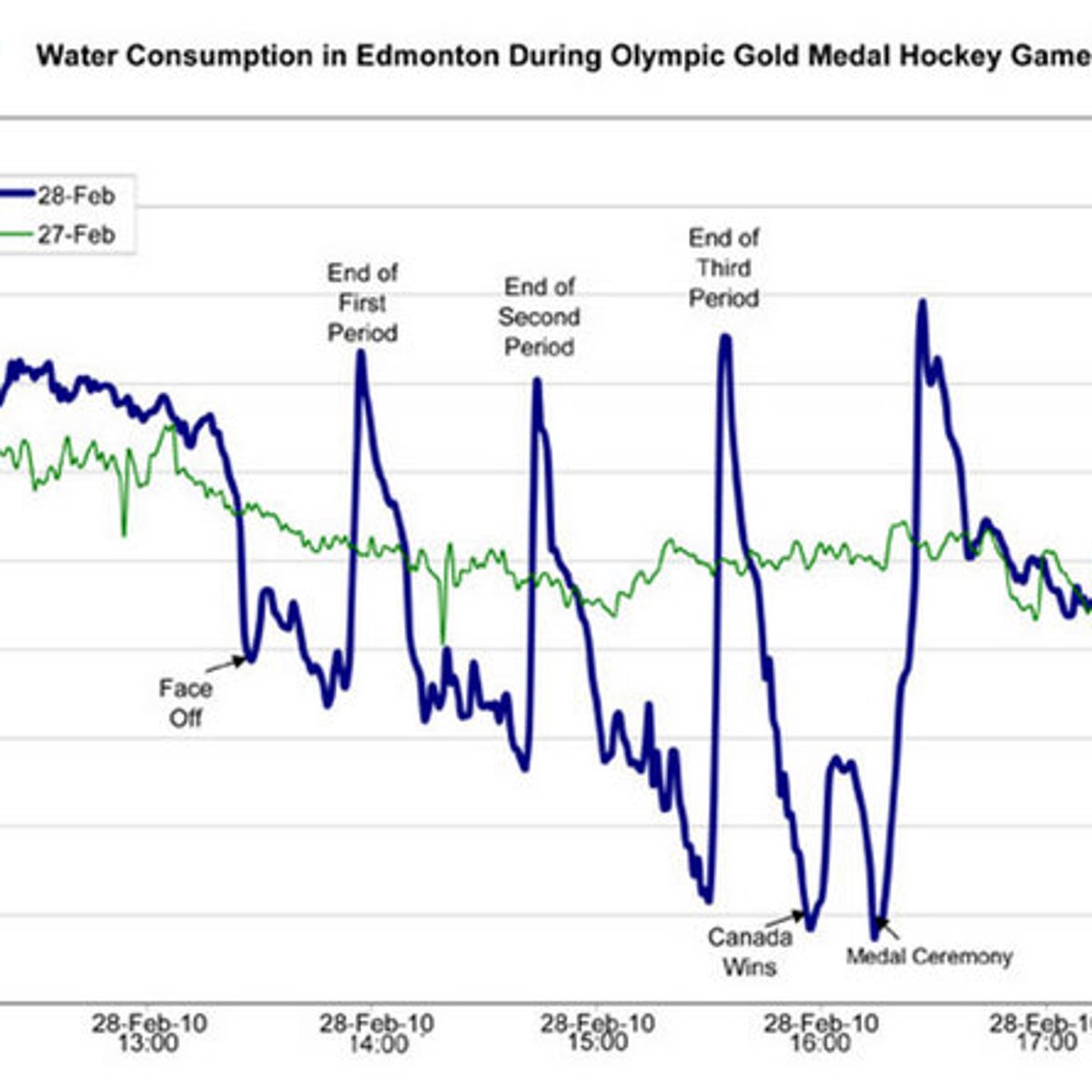
# Lec 2.2 Code
library(fpp3)

# Code block 1 ----
# Compare meta-data of data_tibble and data_tsibble
data_tibble <- tibble(
  Year = 2015:2019,
  Observation = c(123, 39, 78, 52, 110)
)
data_tibble

# Set variable that indexes the data: Year
data_tsibble <- tsibble(data_tibble, index = "Year")
data_tsibble


# Code block 2 ----
# Scatterplot of relationship between two time series
# Code for Fig. 2.14:
vic_elec |>
  filter(year(Time) == 2014) |>
  ggplot(aes(x = Temperature, y = Demand)) +
  geom_point() +
  labs(x = "Temperature (degrees Celsius)",
       y = "Electricity demand (GW)")

# Code for Fig 2.14 with (simplified) notion of time
vic_elec |>
  filter(year(Time) == 2014) |>
  # Add this:
  mutate(month = factor(month(Date))) |>
  # Add color scale
  ggplot(aes(x = Temperature, y = Demand, col = month)) +
  geom_point() +
  labs(x = "Temperature (degrees Celsius)",
       y = "Electricity demand (GW)")
Lec 2.1: Tue 9/12
- Join
#questionschannel on Slack - Fill in your information on roster
- ChatGPT citation mechanism: share link
- Developing a python/jupyter notebook workflow
- Open a jupyter notebook
- Start “Manipulating Time Series Data in Python” DataCamp course, to be completed by Tue 9/19 before class
- Screencast recording here
Lec 1.2: Thu 9/7
Install software and computing: See syllabus