The map() family of
functions
In this lab, we will learn how to use variants of map()
to iterate tasks.
Goal: by the end of this lab, you should be able to
use variants of map() to do complex operations with a few
lines of code.
One input: map()
In this lab, we are going to be generating a bunch of random data.
First, we’re going to create a vector that holds n,
which represents how much random data we are going to generate in each
simulation. We’re going to store this as a tibble with one
column (for now).
random_dist <- tibble(
  n = 1:20 * 100
)
Next, we use the map() function to generate a
list of random vectors, each drawn from a normal
distribution with a different number of samples drawn in each case.
random_data <- map(random_dist$n, rnorm)
str(random_data)
## List of 20
## $ : num [1:100] 0.793 0.522 1.746 -1.271 2.197 ...
## $ : num [1:200] -0.8109 -2.9438 -0.0188 -0.3547 0.0356 ...
## $ : num [1:300] -1.181 -1.228 0.457 -0.251 -0.338 ...
## $ : num [1:400] -0.00654 2.08749 -0.38644 0.75195 1.63085 ...
## $ : num [1:500] 0.0952 -0.0375 0.9213 1.6603 0.7964 ...
## $ : num [1:600] 0.0171 2.5526 -0.0252 0.4658 -0.0748 ...
## $ : num [1:700] -0.857 0.145 0.376 -0.454 -0.247 ...
## $ : num [1:800] -0.899 0.66 -0.212 0.492 0.198 ...
## $ : num [1:900] 0.156 -0.666 -1.518 0.614 -1.704 ...
## $ : num [1:1000] 1.69 -1.048 0.994 -1.896 -0.806 ...
## $ : num [1:1100] 0.733 -0.779 -1.366 -0.726 0.87 ...
## $ : num [1:1200] 0.346 0.487 0.718 1.327 1.016 ...
## $ : num [1:1300] 1.079 -0.963 -0.828 1.548 0.144 ...
## $ : num [1:1400] -1.4 -2.11 1.04 -2.69 -1.07 ...
## $ : num [1:1500] 0.484 0.888 -1.834 1.014 -0.062 ...
## $ : num [1:1600] 1.026 -1.665 -1.001 -0.537 -0.419 ...
## $ : num [1:1700] -1.456 1.223 -0.462 0.588 0.828 ...
## $ : num [1:1800] 1.599 -0.364 -0.612 -1.786 1.263 ...
## $ : num [1:1900] 0.202 -0.291 -0.709 -0.285 -0.485 ...
## $ : num [1:2000] -0.2624 1.5296 -0.0824 -0.4526 1.2523 ...To keep things organized, let’s save the list of random
data to our original tibble. Note that data is
now a list-column.
random_dist$data <- random_data
random_dist
This is compact way (20 rows and 2 columns) to store what are really
21,000 random numbers! You can see the long version by
unnest()-ing.
random_dist %>%
  unnest(cols = data) %>%
  nrow()
## [1] 21000Next, we can perform some rudimentary analysis on each randomly generated data set. Here, we compute the means and standard deviations of each simulated data set.
random_dist <- random_dist %>%
  mutate(
    means = map_dbl(data, mean),
    sds = map_dbl(data, sd)
)- Use the
median()function to compute the median of each data set. Add them to therandom_distdata frame.
# SAMPLE SOLUTION

random_dist <- random_dist %>%
mutate(medians = map_dbl(data, median))- Make a scatterplot of the standard deviations as a function of the size of the simulation. Do you notice a pattern?
# SAMPLE SOLUTION

ggplot(random_dist, aes(x = n, y = sds)) +
  geom_point()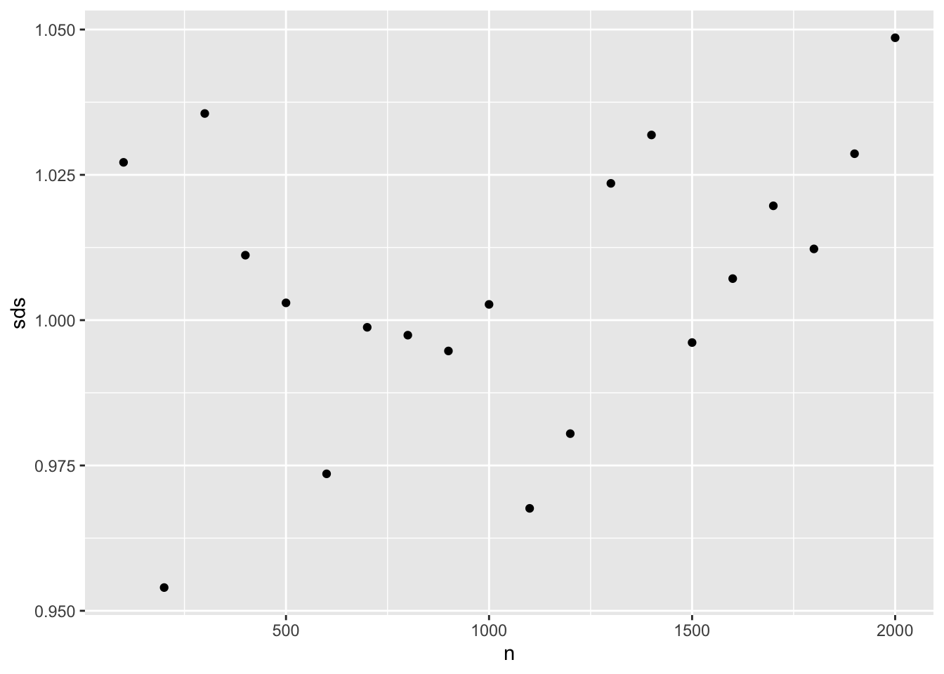
One input, not first argument
In the previous examples, the vector that we were iterating over was the first argument to the function that we wanted to apply. This is typical, but not the only situation we may find ourselves in.
Here, we want to experiment with different trimmed means. That is, we want to compute the mean of a single simulated data set after throwing away either 10% or 25% of the data.
In this case, we want to iterate over the trim argument
to mean() instead of the x argument. To do
this, we make use of the .x syntax made possible by the
~.
map_dbl(
  c(0.1, 0.25),
  ~mean(x = random_dist$data[[1]], trim = .x)
)
## [1] 0.08418324 0.08603153- Suppose we wanted to apply both values for the trimmed mean to
all of the data sets. Why is
map_dbl()insufficient for this task? What kind of function would we need?
Now we’re going to write each one of our data sets to a separate CSV
file. We’ll name each file using the sample size, so that we can tell
them apart later. The path() function from the
fs package will specify the full path. The
tempdir() function returns the path to the temp directory
on your computer.
random_dist <- random_dist %>%
  mutate(
    filename = paste0("random_data_", n, ".csv"),
    file = fs::path(tempdir(), filename)
)
Note that each entry in the data list-column is a double
vector. In order to write a CSV, we need this to be a
data.frame. The enframe() function converts a
vector into a tibble. We can use map() to do
this to each data set.
random_dist <- random_dist %>%
  mutate(data_frame = map(data, enframe))
Multiple inputs
Finally, we’re ready to write the files. Note that we need to know
both the path to the CSV file that we want to create, and the data set
itself. The pwalk() function will step through our data
frame row-by-row. To make things easier, we’ll rename the
data column x, so it matches the argument name
write_csv() is expecting.
args(write_csv)## function (x, file, na = "NA", append = FALSE, col_names = !append,
## quote = c("needed", "all", "none"), escape = c("double",
## "backslash", "none"), eol = "\n", num_threads = readr_threads(),
## progress = show_progress(), path = deprecated(), quote_escape = deprecated())
## NULLrandom_dist %>%
select(x = data_frame, file) %>%
pwalk(write_csv)- Rewrite the previous
pwalk()statement without the renaming (i.e.,select()) step. To do this you will need to use the~formulation.
To confirm that this worked, use fs::dir_ls() to
retrieve the list of CSVs in your temp directory.
csv <- fs::dir_ls(tempdir(), regexp = "\\.csv")
csv
## /var/folders/d_/6fhql14j7hd93zfzcn1x3ttxn8st2y/T/Rtmpopa0Ng/random_data_100.csv
## /var/folders/d_/6fhql14j7hd93zfzcn1x3ttxn8st2y/T/Rtmpopa0Ng/random_data_1000.csv
## /var/folders/d_/6fhql14j7hd93zfzcn1x3ttxn8st2y/T/Rtmpopa0Ng/random_data_1100.csv
## /var/folders/d_/6fhql14j7hd93zfzcn1x3ttxn8st2y/T/Rtmpopa0Ng/random_data_1200.csv
## /var/folders/d_/6fhql14j7hd93zfzcn1x3ttxn8st2y/T/Rtmpopa0Ng/random_data_1300.csv
## /var/folders/d_/6fhql14j7hd93zfzcn1x3ttxn8st2y/T/Rtmpopa0Ng/random_data_1400.csv
## /var/folders/d_/6fhql14j7hd93zfzcn1x3ttxn8st2y/T/Rtmpopa0Ng/random_data_1500.csv
## /var/folders/d_/6fhql14j7hd93zfzcn1x3ttxn8st2y/T/Rtmpopa0Ng/random_data_1600.csv
## /var/folders/d_/6fhql14j7hd93zfzcn1x3ttxn8st2y/T/Rtmpopa0Ng/random_data_1700.csv
## /var/folders/d_/6fhql14j7hd93zfzcn1x3ttxn8st2y/T/Rtmpopa0Ng/random_data_1800.csv
## /var/folders/d_/6fhql14j7hd93zfzcn1x3ttxn8st2y/T/Rtmpopa0Ng/random_data_1900.csv
## /var/folders/d_/6fhql14j7hd93zfzcn1x3ttxn8st2y/T/Rtmpopa0Ng/random_data_200.csv
## /var/folders/d_/6fhql14j7hd93zfzcn1x3ttxn8st2y/T/Rtmpopa0Ng/random_data_2000.csv
## /var/folders/d_/6fhql14j7hd93zfzcn1x3ttxn8st2y/T/Rtmpopa0Ng/random_data_300.csv
## /var/folders/d_/6fhql14j7hd93zfzcn1x3ttxn8st2y/T/Rtmpopa0Ng/random_data_400.csv
## /var/folders/d_/6fhql14j7hd93zfzcn1x3ttxn8st2y/T/Rtmpopa0Ng/random_data_500.csv
## /var/folders/d_/6fhql14j7hd93zfzcn1x3ttxn8st2y/T/Rtmpopa0Ng/random_data_600.csv
## /var/folders/d_/6fhql14j7hd93zfzcn1x3ttxn8st2y/T/Rtmpopa0Ng/random_data_700.csv
## /var/folders/d_/6fhql14j7hd93zfzcn1x3ttxn8st2y/T/Rtmpopa0Ng/random_data_800.csv
## /var/folders/d_/6fhql14j7hd93zfzcn1x3ttxn8st2y/T/Rtmpopa0Ng/random_data_900.csvReversing the process
Another useful application of map() is to read in a
bunch of files. Here, we use the list of CSV paths and
read_csv() to build a large data set of all of the
simulated data. Note that the .id argument to
map_dfr() ensures that the filename is included as a column
in the resulting data frame. Otherwise, we wouldn’t know which data set
came from which file!
all_data <- csv %>%
  map_dfr(read_csv, .id = "filename")

all_data
An application of nest() brings the data back into a
compact form.
nested_data <- all_data %>%
  nest(data = c(name, value))

nested_data
Engagement
Prompt: What questions do you still have about
map()?