Create focal versus competitor trees data frame

"Focal versus competitor trees" data frames are the main data frame used for analysis. "Focal trees" are all trees that satisfy the following criteria

1. Were alive at both censuses

2. Were not part of the study region's buffer as computed by add_buffer_variable()

3. Were not a resprout at the second census. Such trees should be coded as "R" in the codes2 variable (OK if a resprout at first census)

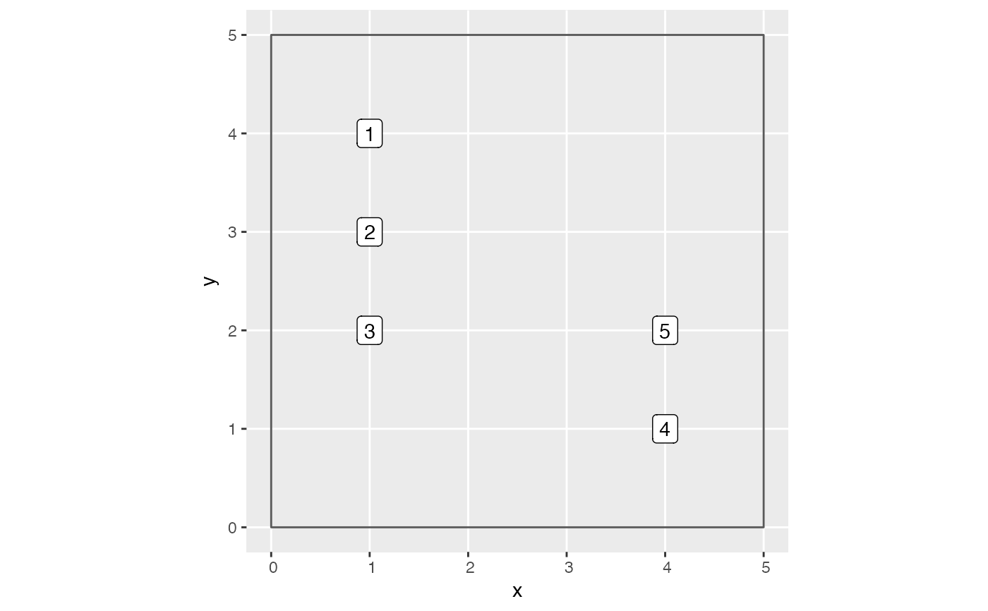
For each focal tree, "competitor trees" are all trees that (1) were alive at the first census and (2) within comp_dist distance of the focal tree.

create_focal_vs_comp(growth_df, comp_dist, blocks, id, comp_x_var)

Arguments

growth_df	A compute_growth() output converted to sf object
comp_dist	Distance to determine which neighboring trees to a focal tree are competitors.
blocks	An sf object of a blockCV block output
id	A character string of the variable name in growth_df uniquely identifying each tree
comp_x_var	A character string indicating which numerical variable to use as competitor explanatory variable

Value

focal_vs_comp data frame of all focal trees and for each focal tree all possible competitor trees. In particular, for each competitor tree we return comp_x_var. Potential examples of comp_x_var include basal area or estimate above ground biomass.

Note

In order to speed computation, in particular of distances between all focal/competitor tree pairs, we use the cross-validation blockCV object to divide the study region into smaller subsets.

See also

Other data processing functions: compute_growth(), create_bayes_lm_data()

Examples

library(ggplot2)
library(dplyr)
library(stringr)
library(sf)
library(sfheaders)
library(tibble)

# Create fold information sf object.
SpatialBlock_ex <-
  tibble(
    # Study region boundary
    x = c(0, 0, 5, 5),
    y = c(0, 5, 5, 0)
  ) %>%
  # Convert to sf object
  sf_polygon() %>%
  mutate(folds = "1")

# Plot example data. Observe for comp_dist = 1.5, there are 6 focal vs comp pairs:
# 1. focal 1 vs comp 2
# 2. focal 2 vs comp 1
# 3. focal 2 vs comp 3
# 4. focal 3 vs comp 2
# 5. focal 4 vs comp 5
# 6. focal 5 vs comp 4
ggplot() +
  geom_sf(data = SpatialBlock_ex, fill = "transparent") +
  geom_sf_label(data = growth_toy, aes(label = ID))

# Return corresponding data frame
growth_toy %>%
  mutate(basal_area = 0.0001 * pi * (dbh1 / 2)^2) %>%
  create_focal_vs_comp(comp_dist = 1.5, blocks = SpatialBlock_ex, id = "ID",
                       comp_x_var = "basal_area")
#> # A tibble: 5 × 7
#>   focal_ID focal_sp       dbh foldID geometry growth comp            
#>      <int> <fct>        <dbl> <fct>   <POINT>  <dbl> <list>          
#> 1        1 tulip poplar    40 1         (1 4)      1 <tibble [1 × 4]>
#> 2        2 red oak         25 1         (1 3)      2 <tibble [2 × 4]>
#> 3        3 red oak         30 1         (1 2)      1 <tibble [1 × 4]>
#> 4        4 tulip poplar    35 1         (4 1)      3 <tibble [1 × 4]>
#> 5        5 tulip poplar    20 1         (4 2)      2 <tibble [1 × 4]>

# Load in growth_df with spatial data
# See ?growth_ex for attaching spatial data to growth_df
data(growth_spatial_ex)
# Load in blocks
data(blocks_ex)

focal_vs_comp_ex <- growth_spatial_ex %>%
  mutate(basal_area = 0.0001 * pi * (dbh1 / 2)^2) %>%
  create_focal_vs_comp(comp_dist = 1, blocks = blocks_ex, id = "ID",
                       comp_x_var = "basal_area")