Example growth data frame with spatial data for small example

This is an example growth data frame formed from two census data frames which has been updated with spatial data. It starts from growth_ex.

growth_spatial_ex

Format

A sf spatial tibble

ID

Tree identification number. This identifies an individual tree and can be used to connect trees between the two censuses.

sp

Species of the individual

codes1

Code for additional information on the stem during the first census: M means the main stem of the individual tree and R means the stem was lost, but the tag was moved to another stem greater than DBH cutoff, this stands for resprout.

dbh1

Diameter at breast height of the tree in cm at the first census

dbh2

Diameter at breast height of the tree in cm at the second census

growth

Average annual growth between the two censuses in cm per year

codes2

Codes at the second census

geometry

Point location of the individual

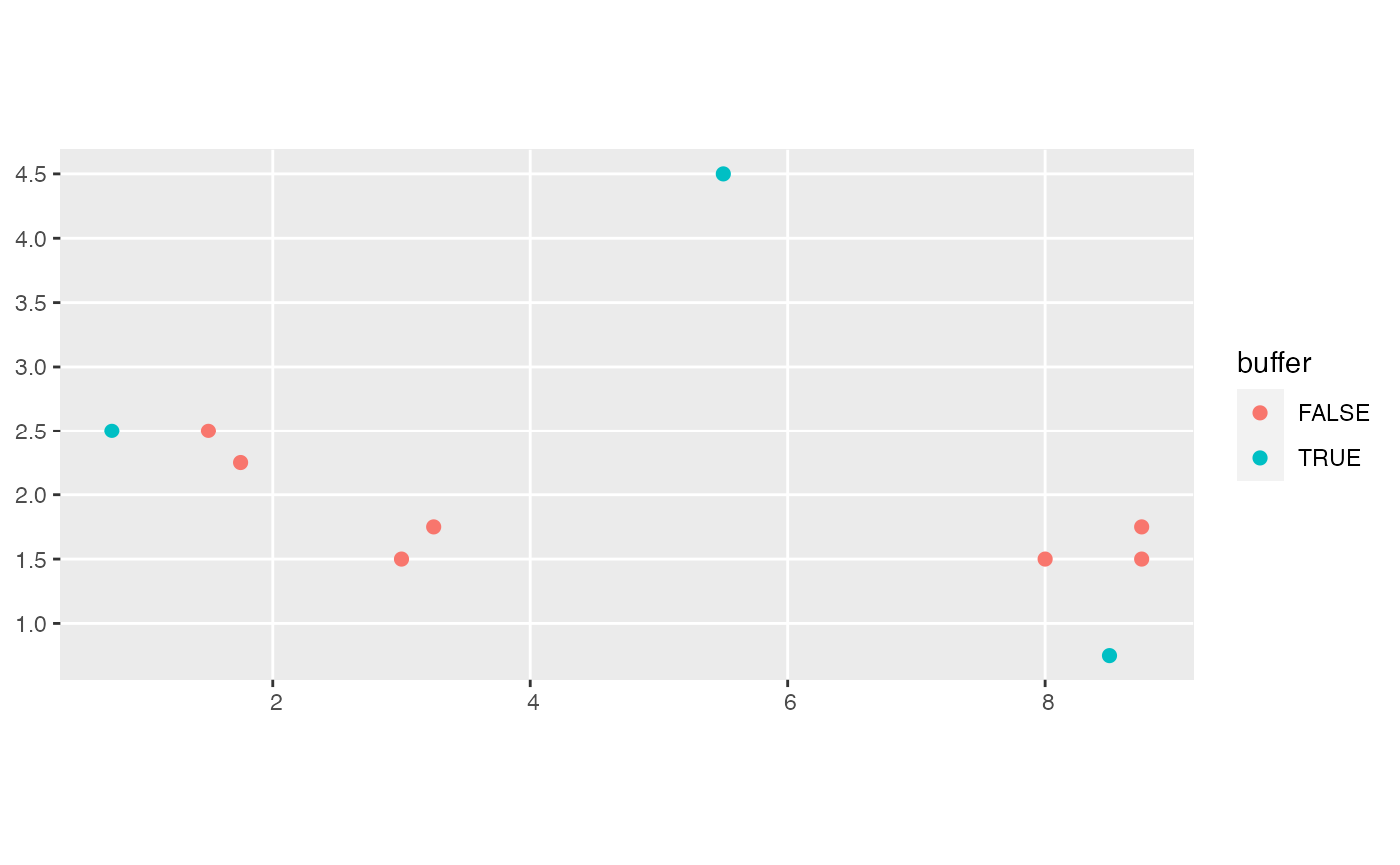
buffer

A boolean variable for whether the individual is in the buffer region or not

foldID

Which cross-validation fold the individual is in

See also

compute_growth()

Other example data objects: blocks_ex, census_1_ex, census_2008_bw, census_2014_bw, census_2_ex, comp_bayes_lm_ex, focal_vs_comp_ex, growth_ex, growth_toy, species_bw, study_region_bw, study_region_ex

Examples

library(ggplot2)
library(dplyr)
library(sf)

comp_dist <- 1

ggplot() +
  geom_sf(data = growth_spatial_ex, aes(col = buffer), size = 2)

ggplot() +
  geom_sf(data = growth_spatial_ex, aes(col = foldID), size = 2)

# Create the focal versus comp data frame
focal_vs_comp_ex <- growth_spatial_ex %>%
  mutate(basal_area = 0.0001 * pi * (dbh1 / 2)^2) %>%
  create_focal_vs_comp(comp_dist, blocks = blocks_ex, id = "ID", comp_x_var = "basal_area")